Teacher Observation Correlation
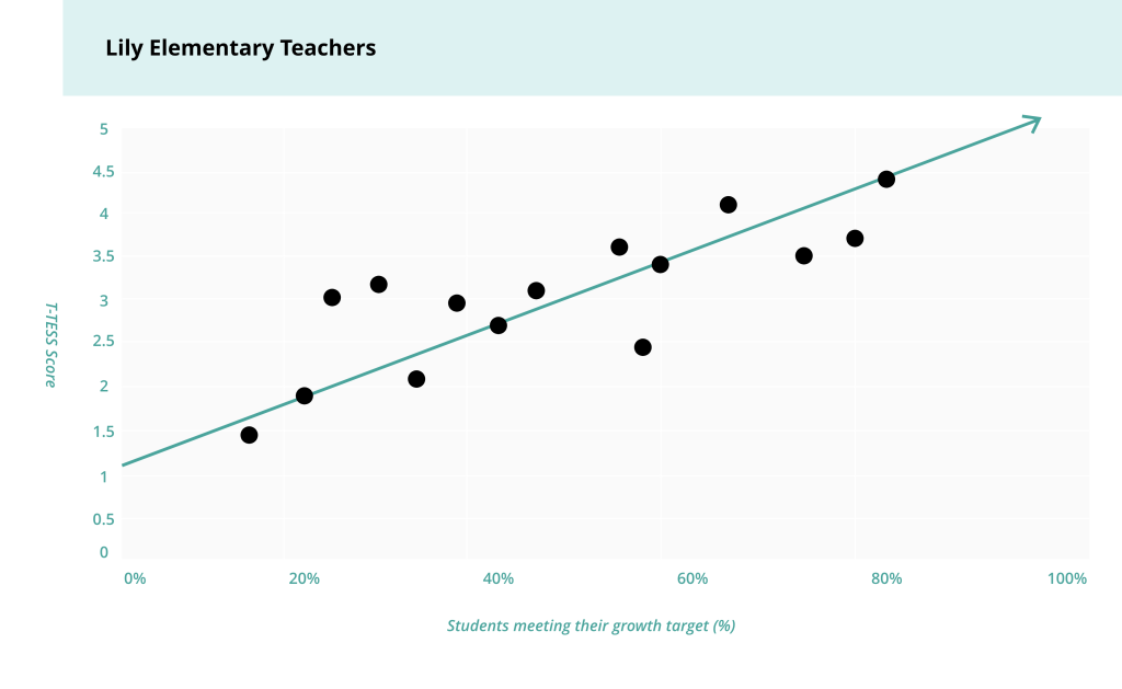
Long Description of T-TESS scores graphic showing positive correlation between teacher observation scores and student growth.
This scatterplot graph has T-TESS scores on the Y-axis (zero to five in increments of 0.5) and on the X-axis is percentage of students meeting their growth targets in increments of 20%. Each dot on the graph represents one teacher. For example, there is one dot that shows a that one teacher had a T-TESS score of two and 20% of that teachers students met their growth target. The dots form a loose line moving up and to the right. There is a line on the graph demonstrating that the dots move up and to the right. Generally, the higher a teacher’s T-TESS score, the higher the percentage of their students meeting their growth target. This graph shows a positive correlation between teachers’ observation scores and the percentage of students meeting their growth targets.
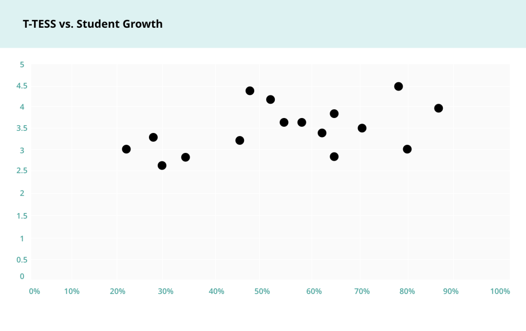
Long Description of T-TESS scores graphic showing no correlation between teacher observation scores and student growth.
This scatterplot graph has T-TESS scores on the Y-axis (zero to five in increments of 0.5) and on the X-axis is percentage of students meeting their growth targets in increments of 20%. Each dot on the graph represents one teacher. For example, there is one dot that shows a that one teacher had a T-TESS score of four and 20% of that teachers students met their growth target. On this graph, the dots do not form a line. Teachers with higher T-TESS scores are not generally getting more or less students to meet their growth targets than teachers with lower T-TESS scores. This graph shows no correlation between teachers’ observation scores and the percentage of students meeting their growth targets.

Long Description of explaining the Correlation Coefficient.
This image shows a series of seven scatterplots. Furthest to the left is a scatterplot in which all the dots are on a perfect line moving from upper left to lower right. This graph shows a perfect negative correlation, represented by a correlation coefficient of -1. The next two graphs moving to the right also show a negative correlation with dots moving from the top left to the bottom right, but these graphs have weaker negative correlation coefficients of -0.9 and -0.5 respectively. When connected to teacher observation and student growth, these graphs show a scenario in which student growth decreases as observation scores increase. The middle graph moving to the right shows no correlation, or a correlation coefficient of zero. There is no pattern in the dots. Moving to the right the dots on the next three graphs show progressively stronger positive correlation. Graph five has a correlation of 0.5 with dots moving in a loose pattern from the lower left to the upper right. Graph six has a correlation of 0.9 with dots moving in a stronger pattern from the lower left to the upper right. Graph seven has a perfect positive correlation of 1 with dots on a perfect line moving from the lower left to the upper right. When connected to teacher observation and student growth, graphs five through seven show a scenario in which student growth increases as teacher observation scores increase. It is the district’s goal to have a correlation coefficient of 0.24 which represents a moderate positive correlation.


Long Description of How to Calculate Correlation Coefficient
This image shows a screen shot of three columns on an excel spreadsheet. The first column is Teacher. There are 17 rows and each row under the Teacher header has a different letter from A to P to label individual teachers. The next column is T-TESS Score. There is a T-TESS score associated with each corresponding teacher on the row in this column. The last column is percentage of students meeting growth targets. There is a growth percentage associated with each corresponding teacher on the row in this column. At the bottom of this third column is the excel formula for correlation coefficient which is =correl(B2:B17, C2:C17). The purpose of this photo is to show how to calculate correlation coefficient using Microsoft Excel.

Long Description of How to Calculate Correlation Coefficient, part 2
This image shows the same Excel spreadsheet as the previous image. The only difference is in the cell where the formula was, now appears the actual correlation coefficient. In this example the correlation coefficient is rounded to 0.48.

Long Description of a positive correlation in teacher observation ratings increase and student growth ratings increase.
This scatter plot is a visual representation of the data shown in the Excel spreadsheet in the previous two images. On the Y-axis is T-TESS scores from zero to five. On X-axis is percentage of students meeting their growth target from 0% to 100%. The dots form a loose line up and to the right showing a positive correlation.